
Amazon MLS-C01 Practice Exams
Last updated on Oct 23,2026- Exam Code: MLS-C01
- Exam Name: AWS Certified Machine Learning - Specialty
- Certification Provider: Amazon
- Latest update: Oct 23,2026
A Machine Learning Specialist must build out a process to query a dataset on Amazon S3 using Amazon Athena. The dataset contains more than 800.000 records stored as plaintext CSV files Each record contains 200 columns and is approximately 1 5 MB in size Most queries will span 5 to 10 columns only.
How should the Machine Learning Specialist transform the dataset to minimize query runtime?
- A . Convert the records to Apache Parquet format
- B . Convert the records to JSON format
- C . Convert the records to GZIP CSV format
- D . Convert the records to XML format
A
Explanation:
Explanation:
Amazon Athena is an interactive query service that allows you to analyze data stored in Amazon S3 using standard SQL. Athena is serverless, so you only pay for the queries that you run and there is no infrastructure to manage.
To optimize the query performance of Athena, one of the best practices is to convert the data into a columnar format, such as Apache Parquet or Apache ORC. Columnar formats store data by columns rather than by rows, which allows Athena to scan only the columns that are relevant to the query, reducing the amount of data read and improving the query speed. Columnar formats also support compression and encoding schemes that can reduce the storage space and the data scanned per query, further enhancing the performance and reducing the cost.
In contrast, plaintext CSV files store data by rows, which means that Athena has to scan the entire row even if only a few columns are needed for the query. This increases the amount of data read and the query latency. Moreover, plaintext CSV files do not support compression or encoding, which means that they take up more storage space and incur higher query costs.
Therefore, the Machine Learning Specialist should transform the dataset to Apache Parquet format
to minimize query runtime.
References:
Top 10 Performance Tuning Tips for Amazon Athena
Columnar Storage Formats
Using compressions will reduce the amount of data scanned by Amazon Athena, and also reduce your S3 bucket storage. It’s a Win-Win for your AWS bill. Supported formats: GZIP, LZO, SNAPPY (Parquet) and ZLIB.
Reference: https://www.cloudforecast.io/blog/using-parquet-on-athena-to-save-money-on-aws/
A Machine Learning Specialist works for a credit card processing company and needs to predict which transactions may be fraudulent in near-real time. Specifically, the Specialist must train a model that returns the probability that a given transaction may fraudulent.
How should the Specialist frame this business problem?
- A . Streaming classification
- B . Binary classification
- C . Multi-category classification
- D . Regression classification
B
Explanation:
The business problem of predicting whether a new credit card applicant will default on a credit card payment can be framed as a binary classification problem. Binary classification is the task of predicting a discrete class label output for an example, where the class label can only take one of two possible values. In this case, the class label can be either “default” or “no default”, indicating whether the applicant will or will not default on a credit card payment. A binary classification model can return the probability that a given applicant belongs to each class, and then assign the applicant to the class with the highest probability. For example, if the model predicts that an applicant has a 0.8 probability of defaulting and a 0.2 probability of not defaulting, then the model will classify the applicant as “default”. Binary classification is suitable for this problem because the outcome of interest is categorical and binary, and the model needs to return the probability of each outcome.
References:
AWS Machine Learning Specialty Exam Guide
AWS Machine Learning Training – Classification vs Regression in Machine Learning
An online reseller has a large, multi-column dataset with one column missing 30% of its data A Machine Learning Specialist believes that certain columns in the dataset could be used to reconstruct the missing data.
Which reconstruction approach should the Specialist use to preserve the integrity of the dataset?
- A . Listwise deletion
- B . Last observation carried forward
- C . Multiple imputation
- D . Mean substitution
C
Explanation:
Multiple imputation is a technique that uses machine learning to generate multiple plausible values for each missing value in a dataset, based on the observed data and the relationships among the variables. Multiple imputation preserves the integrity of the dataset by accounting for the uncertainty and variability of the missing data, and avoids the bias and loss of information that may result from other methods, such as listwise deletion, last observation carried forward, or mean substitution. Multiple imputation can improve the accuracy and validity of statistical analysis and machine learning models that use the imputed dataset.
References:
Managing missing values in your target and related datasets with automated imputation support in Amazon Forecast
Imputation by feature importance (IBFI): A methodology to impute missing data in large datasets Multiple Imputation by Chained Equations (MICE) Explained
A data scientist is working on a public sector project for an urban traffic system. While studying the traffic patterns, it is clear to the data scientist that the traffic behavior at each light is correlated, subject to a small stochastic error term. The data scientist must model the traffic behavior to analyze the traffic patterns and reduce congestion.
How will the data scientist MOST effectively model the problem?
- A . The data scientist should obtain a correlated equilibrium policy by formulating this problem as a multi-agent reinforcement learning problem.
- B . The data scientist should obtain the optimal equilibrium policy by formulating this problem as a single-agent reinforcement learning problem.
- C . Rather than finding an equilibrium policy, the data scientist should obtain accurate predictors of traffic flow by using historical data through a supervised learning approach.
- D . Rather than finding an equilibrium policy, the data scientist should obtain accurate predictors of traffic flow by using unlabeled simulated data representing the new traffic patterns in the city and applying an unsupervised learning approach.
A
Explanation:
The data scientist should obtain a correlated equilibrium policy by formulating this problem as a multi-agent reinforcement learning problem.
This is because:
Multi-agent reinforcement learning (MARL) is a subfield of reinforcement learning that deals with learning and coordination of multiple agents that interact with each other and the environment 1. MARL can be applied to problems that involve distributed decision making, such as traffic signal control, where each traffic light can be modeled as an agent that observes the traffic state and chooses an action (e.g., changing the signal phase) to optimize a reward function (e.g., minimizing the delay or congestion) 2.
A correlated equilibrium is a solution concept in game theory that generalizes the notion of Nash equilibrium. It is a probability distribution over the joint actions of the agents that satisfies the following condition: no agent can improve its expected payoff by deviating from the distribution, given that it knows the distribution and the actions of the other agents 3. A correlated equilibrium can capture the correlation among the agents’ actions, which is useful for modeling the traffic behavior at each light that is subject to a small stochastic error term.
A correlated equilibrium policy is a policy that induces a correlated equilibrium in a MARL setting. It can be obtained by using various methods, such as policy gradient, actor-critic, or Q-learning algorithms, that can learn from the feedback of the environment and the communication among the agents 4. A correlated equilibrium policy can achieve a better performance than a Nash equilibrium policy, which assumes that the agents act independently and ignore the correlation among their actions 5.
Therefore, by obtaining a correlated equilibrium policy by formulating this problem as a MARL problem, the data scientist can most effectively model the traffic behavior and reduce congestion.
References:
Multi-Agent Reinforcement Learning Multi-Agent Reinforcement Learning for Traffic Signal Control: A Survey Correlated Equilibrium
Multi-Agent Actor-Critic for Mixed Cooperative-Competitive Environments Correlated Q-Learning
A manufacturing company needs to identify returned smartphones that have been damaged by moisture. The company has an automated process that produces 2.000 diagnostic values for each phone. The database contains more than five million phone evaluations. The evaluation process is consistent, and there are no missing values in the data. A machine learning (ML) specialist has trained an Amazon SageMaker linear learner ML model to classify phones as moisture damaged or not moisture damaged by using all available features. The model’s F1 score is 0.6.
What changes in model training would MOST likely improve the model’s F1 score? (Select TWO.)
- A . Continue to use the SageMaker linear learner algorithm. Reduce the number of features with the SageMaker principal component analysis (PCA) algorithm.
- B . Continue to use the SageMaker linear learner algorithm. Reduce the number of features with the scikit-iearn multi-dimensional scaling (MDS) algorithm.
- C . Continue to use the SageMaker linear learner algorithm. Set the predictor type to regressor.
- D . Use the SageMaker k-means algorithm with k of less than 1.000 to train the model
- E . Use the SageMaker k-nearest neighbors (k-NN) algorithm. Set a dimension reduction target of less than 1,000 to train the model.
AE
Explanation:
Option A is correct because reducing the number of features with the SageMaker PCA algorithm can help remove noise and redundancy from the data, and improve the model’s performance. PCA is a dimensionality reduction technique that transforms the original features into a smaller set of linearly uncorrelated features called principal components. The SageMaker linear learner algorithm supports PCA as a built-in feature transformation option.
Option E is correct because using the SageMaker k-NN algorithm with a dimension reduction target of less than 1,000 can help the model learn from the similarity of the data points, and improve the model’s performance. k-NN is a non-parametric algorithm that classifies an input based on the majority vote of its k nearest neighbors in the feature space. The SageMaker k-NN algorithm supports dimension reduction as a built-in feature transformation option.
Option B is incorrect because using the scikit-learn MDS algorithm to reduce the number of features is not a feasible option, as MDS is a computationally expensive technique that does not scale well to large datasets. MDS is a dimensionality reduction technique that tries to preserve the pairwise distances between the original data points in a lower-dimensional space.
Option C is incorrect because setting the predictor type to regressor would change the model’s objective from classification to regression, which is not suitable for the given problem. A regressor model would output a continuous value instead of a binary label for each phone.
Option D is incorrect because using the SageMaker k-means algorithm with k of less than 1,000
would not help the model classify the phones, as k-means is a clustering algorithm that groups the
data points into k clusters based on their similarity, without using any labels. A clustering model
would not output a binary label for each phone.
References:
Amazon SageMaker Linear Learner Algorithm
Amazon SageMaker K-Nearest Neighbors (k-NN) Algorithm [Principal Component Analysis – Scikit-learn] [Multidimensional Scaling – Scikit-learn]
A data scientist is trying to improve the accuracy of a neural network classification model. The data scientist wants to run a large hyperparameter tuning job in Amazon SageMaker.
However, previous smaller tuning jobs on the same model often ran for several weeks. The ML specialist wants to reduce the computation time required to run the tuning job.
Which actions will MOST reduce the computation time for the hyperparameter tuning job? (Select TWO.)
- A . Use the Hyperband tuning strategy.
- B . Increase the number of hyperparameters.
- C . Set a lower value for the MaxNumberOfTrainingJobs parameter.
- D . Use the grid search tuning strategy
- E . Set a lower value for the MaxParallelTrainingJobs parameter.
AC
Explanation:
The Hyperband tuning strategy is a multi-fidelity based tuning strategy that dynamically reallocates resources to the most promising hyperparameter configurations. Hyperband uses both intermediate and final results of training jobs to stop under-performing jobs and reallocate epochs to well-utilized
hyperparameter configurations. Hyperband can provide up to three times faster hyperparameter tuning compared to other strategies1. Setting a lower value for the MaxNumberOfTrainingJobs parameter can also reduce the computation time for the hyperparameter tuning job by limiting the number of training jobs that the tuning job can launch. This can help avoid unnecessary or redundant training jobs that do not improve the objective metric.
The other options are not effective ways to reduce the computation time for the hyperparameter tuning job. Increasing the number of hyperparameters will increase the complexity and dimensionality of the search space, which can result in longer computation time and lower performance. Using the grid search tuning strategy will also increase the computation time, as grid search methodically searches through every combination of hyperparameter values, which can be very expensive and inefficient for large search spaces. Setting a lower value for the MaxParallelTrainingJobs parameter will reduce the number of training jobs that can run in parallel, which can slow down the tuning process and increase the waiting time.
References:
• How Hyperparameter Tuning Works
• Best Practices for Hyperparameter Tuning
• HyperparameterTuner
• Amazon SageMaker Automatic Model Tuning now provides up to three times faster hyperparameter tuning with Hyperband
A data scientist at a financial services company used Amazon SageMaker to train and deploy a model that predicts loan defaults. The model analyzes new loan applications and predicts the risk of loan default. To train the model, the data scientist manually extracted loan data from a database. The data scientist performed the model training and deployment steps in a Jupyter notebook that is hosted on SageMaker Studio notebooks. The model’s prediction accuracy is decreasing over time.
Which combination of slept in the MOST operationally efficient way for the data scientist to maintain the model’s accuracy? (Select TWO.)
- A . Use SageMaker Pipelines to create an automated workflow that extracts fresh data, trains the model, and deploys a new version of the model.
- B . Configure SageMaker Model Monitor with an accuracy threshold to check for model drift. Initiate an Amazon CloudWatch alarm when the threshold is exceeded. Connect the workflow in SageMaker Pipelines with the CloudWatch alarm to automatically initiate retraining.
- C . Store the model predictions in Amazon S3 Create a daily SageMaker Processing job that reads the predictions from Amazon S3, checks for changes in model prediction accuracy, and sends an email notification if a significant change is detected.
- D . Rerun the steps in the Jupyter notebook that is hosted on SageMaker Studio notebooks to retrain the model and redeploy a new version of the model.
- E . Export the training and deployment code from the SageMaker Studio notebooks into a Python script. Package the script into an Amazon Elastic Container Service (Amazon ECS) task that an AWS Lambda function can initiate.
AB
Explanation:
Option A is correct because SageMaker Pipelines is a service that enables you to create and manage automated workflows for your machine learning projects. You can use SageMaker Pipelines to orchestrate the steps of data extraction, model training, and model deployment in a repeatable and scalable way1.
Option B is correct because SageMaker Model Monitor is a service that monitors the quality of your models in production and alerts you when there are deviations in the model quality. You can use SageMaker Model Monitor to set an accuracy threshold for your model and configure a CloudWatch alarm that triggers when the threshold is exceeded. You can then connect the alarm to the workflow in SageMaker Pipelines to automatically initiate retraining and deployment of a new version of the model2.
Option C is incorrect because it is not the most operationally efficient way to maintain the model’s accuracy. Creating a daily SageMaker Processing job that reads the predictions from Amazon S3 and checks for changes in model prediction accuracy is a manual and time-consuming process. It also requires you to write custom code to perform the data analysis and send the email notification. Moreover, it does not automatically retrain and deploy the model when the accuracy drops. Option D is incorrect because it is not the most operationally efficient way to maintain the model’s accuracy. Rerunning the steps in the Jupyter notebook that is hosted on SageMaker Studio notebooks to retrain the model and redeploy a new version of the model is a manual and error-prone process. It also requires you to monitor the model’s performance and initiate the retraining and deployment steps yourself. Moreover, it does not leverage the benefits of SageMaker Pipelines and SageMaker Model Monitor to automate and streamline the workflow.
Option E is incorrect because it is not the most operationally efficient way to maintain the model’s accuracy. Exporting the training and deployment code from the SageMaker Studio notebooks into a Python script and packaging the script into an Amazon ECS task that an AWS Lambda function can initiate is a complex and cumbersome process. It also requires you to manage the infrastructure and resources for the Amazon ECS task and the AWS Lambda function. Moreover, it does not leverage the benefits of SageMaker Pipelines and SageMaker Model Monitor to automate and streamline the workflow.
References:
1: SageMaker Pipelines – Amazon SageMaker
2: Monitor data and model quality – Amazon SageMaker
A car company is developing a machine learning solution to detect whether a car is present in an image. The image dataset consists of one million images. Each image in the dataset is 200 pixels in height by 200 pixels in width. Each image is labeled as either having a car or not having a car.
Which architecture is MOST likely to produce a model that detects whether a car is present in an image with the highest accuracy?
- A . Use a deep convolutional neural network (CNN) classifier with the images as input. Include a linear output layer that outputs the probability that an image contains a car.
- B . Use a deep convolutional neural network (CNN) classifier with the images as input. Include a softmax output layer that outputs the probability that an image contains a car.
- C . Use a deep multilayer perceptron (MLP) classifier with the images as input. Include a linear output layer that outputs the probability that an image contains a car.
- D . Use a deep multilayer perceptron (MLP) classifier with the images as input. Include a softmax output layer that outputs the probability that an image contains a car.
A
Explanation:
A deep convolutional neural network (CNN) classifier is a suitable architecture for image classification tasks, as it can learn features from the images and reduce the dimensionality of the input. A linear output layer that outputs the probability that an image contains a car is appropriate for a binary classification problem, as it can produce a single scalar value between 0 and 1. A softmax output layer is more suitable for a multi-class classification problem, as it can produce a vector of probabilities that sum up to 1. A deep multilayer perceptron (MLP) classifier is not as effective as a CNN for image classification, as it does not exploit the spatial structure of the images and requires a large number of parameters to process the high-dimensional input.
References:
AWS Certified Machine Learning – Specialty Exam Guide
AWS Training – Machine Learning on AWS
AWS Whitepaper – An Overview of Machine Learning on AWS
A Machine Learning Specialist is working with multiple data sources containing billions of records that need to be joined.
What feature engineering and model development approach should the Specialist take with a dataset this large?
- A . Use an Amazon SageMaker notebook for both feature engineering and model development
- B . Use an Amazon SageMaker notebook for feature engineering and Amazon ML for model development
- C . Use Amazon EMR for feature engineering and Amazon SageMaker SDK for model development
- D . Use Amazon ML for both feature engineering and model development.
C
Explanation:
Amazon EMR is a service that can process large amounts of data efficiently and cost-effectively. It can run distributed frameworks such as Apache Spark, which can perform feature engineering on big data. Amazon SageMaker SDK is a Python library that can interact with Amazon SageMaker service to train and deploy machine learning models. It can also use Amazon EMR as a data source for training data.
References:
Amazon EMR
Amazon SageMaker SDK
Given the following confusion matrix for a movie classification model, what is the true class frequency for Romance and the predicted class frequency for Adventure?
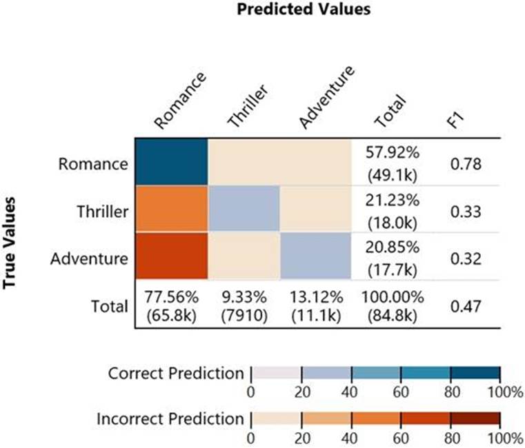
- A . The true class frequency for Romance is 77.56% and the predicted class frequency for Adventure is 20 85%
- B . The true class frequency for Romance is 57.92% and the predicted class frequency for Adventure is 1312%
- C . The true class frequency for Romance is 0 78 and the predicted class frequency for Adventure is (0 47 – 0.32).
- D . The true class frequency for Romance is 77.56% * 0.78 and the predicted class frequency for Adventure is 20 85% ‘ 0.32
B
Explanation:
The true class frequency for Romance is the percentage of movies that are actually Romance out of all the movies. This can be calculated by dividing the sum of the true values for Romance by the total number of movies. The predicted class frequency for Adventure is the percentage of movies that are predicted to be Adventure out of all the movies. This can be calculated by dividing the sum of the predicted values for Adventure by the total number of movies. Based on the confusion matrix, the true class frequency for Romance is 57.92% and the predicted class frequency for Adventure is 13.12%.
References: Confusion Matrix, Classification Metrics