
Google Professional Machine Learning Engineer Practice Exams
Last updated on Oct 10,2026- Exam Code: Professional Machine Learning Engineer
- Exam Name: Google Professional Machine Learning Engineer
- Certification Provider: Google
- Latest update: Oct 10,2026
You developed a Vertex Al ML pipeline that consists of preprocessing and training steps and each set of steps runs on a separate custom Docker image Your organization uses GitHub and GitHub Actions as CI/CD to run unit and integration tests You need to automate the model retraining workflow so that it can be initiated both manually and when a new version of the code is merged in the main branch You want to minimize the steps required to build the workflow while also allowing for maximum flexibility How should you configure the CI/CD workflow?
- A . Trigger a Cloud Build workflow to run tests build custom Docker images, push the images to Artifact Registry and launch the pipeline in Vertex Al Pipelines.
- B . Trigger GitHub Actions to run the tests launch a job on Cloud Run to build custom Docker images push the images to Artifact Registry and launch the pipeline in Vertex Al Pipelines.
- C . Trigger GitHub Actions to run the tests build custom Docker images push the images to Artifact Registry, and launch the pipeline in Vertex Al Pipelines.
- D . Trigger GitHub Actions to run the tests launch a Cloud Build workflow to build custom Dicker images, push the images to Artifact Registry, and launch the pipeline in Vertex Al Pipelines.
D
Explanation:
The best option for automating the model retraining workflow is to use GitHub Actions and Cloud Build. GitHub Actions is a service that can create and run workflows for continuous integration and continuous delivery (CI/CD) on GitHub. GitHub Actions can run tests, build and deploy code, and trigger other actions based on events such as code changes, pull requests, or manual triggers. Cloud Build is a service that can create and run scalable and reliable pipelines to build, test, and deploy software on Google Cloud. Cloud Build can build custom Docker images, push the images to Artifact Registry, and launch the pipeline in Vertex AI Pipelines. Vertex AI Pipelines is a service that can orchestrate machine learning (ML) workflows using Vertex AI. Vertex AI Pipelines can run preprocessing and training steps on custom Docker images, and evaluate, deploy, and monitor the ML model. By using GitHub Actions and Cloud Build, users can leverage the power and flexibility of Google Cloud to automate the model retraining workflow, while minimizing the steps required to build the workflow.
The other options are not as good as option D, for the following reasons:
Option A: Triggering a Cloud Build workflow to run tests, build custom Docker images, push the images to Artifact Registry, and launch the pipeline in Vertex AI Pipelines would require more configuration and maintenance than using GitHub Actions and Cloud Build. Cloud Build is a service that can create and run pipelines to build, test, and deploy software on Google Cloud, but it is not designed to integrate with GitHub or other source code repositories. To trigger a Cloud Build workflow from GitHub, users would need to set up a webhook, a Cloud Pub/Sub topic, and a Cloud Function1. Moreover, Cloud Build does not support manual triggers, which limits the flexibility of the workflow2.
Option B: Triggering GitHub Actions to run the tests, launching a job on Cloud Run to build custom Docker images, pushing the images to Artifact Registry, and launching the pipeline in Vertex AI Pipelines would require more steps and resources than using GitHub Actions and Cloud Build. Cloud Run is a service that can run stateless containers on a fully managed environment or on Anthos. Cloud Run can build custom Docker images, but it is not optimized for this task. Users would need to write a Dockerfile, a cloudbuild.yaml file, and a Cloud Run service configuration file, and use the gcloud command-line tool to build and deploy the image3. Moreover, Cloud Run is designed for serving HTTP requests, not for running ML pipelines, which can have different performance and scalability requirements.
Option C: Triggering GitHub Actions to run the tests, building custom Docker images, pushing the images to Artifact Registry, and launching the pipeline in Vertex AI Pipelines would require more skills and tools than using GitHub Actions and Cloud Build. GitHub Actions can run tests and build code, but it is not specialized for building Docker images. Users would need to install and configure Docker on the GitHub Actions runner, write a Dockerfile, and use the docker command-line tool to build and push the image. Moreover, GitHub Actions has limitations on the disk space, memory, and CPU of the runner, which can affect the speed and reliability of the image building process.
Reference: Building CI/CD for Vertex AI pipelines: The first solution
Cloud Build
GitHub Actions
Vertex AI Pipelines
Triggering builds from GitHub
Triggering builds manually
Building containers
Cloud Run
[Building and testing Docker images with GitHub Actions] [Usage limits, billing, and administration]
You developed a custom model by using Vertex Al to forecast the sales of your company s products based on historical transactional data You anticipate changes in the feature distributions and the correlations between the features in the near future You also expect to receive a large volume of prediction requests You plan to use Vertex Al Model Monitoring for drift detection and you want to minimize the cost.
What should you do?
- A . Use the features for monitoring Set a monitoring- frequency value that is higher than the default.
- B . Use the features for monitoring Set a prediction-sampling-rare value that is closer to 1 than 0.
- C . Use the features and the feature attributions for monitoring. Set a monitoring-frequency value that is lower than the default.
- D . Use the features and the feature attributions for monitoring Set a prediction-sampling-rate value that is closer to 0 than 1.
D
Explanation:
The best option for using Vertex AI Model Monitoring for drift detection and minimizing the cost is to use the features and the feature attributions for monitoring, and set a prediction-sampling-rate value that is closer to 0 than 1. This option allows you to leverage the power and flexibility of Google Cloud to detect feature drift in the input predict requests for custom models, and reduce the storage and computation costs of the model monitoring job. Vertex AI Model Monitoring is a service that can track and compare the results of multiple machine learning runs. Vertex AI Model Monitoring can monitor the model’s prediction input data for feature skew and drift. Feature drift occurs when the feature data distribution in production changes over time. If the original training data is not available, you can enable drift detection to monitor your models for feature drift. Vertex AI Model Monitoring uses TensorFlow Data Validation (TFDV) to calculate the distributions and distance scores for each feature, and compares them with a baseline distribution. The baseline distribution is the statistical distribution of the feature’s values in the training data. If the training data is not available, the baseline distribution is calculated from the first 1000 prediction requests that the model receives. If the distance score for a feature exceeds an alerting threshold that you set, Vertex AI Model Monitoring sends you an email alert. However, if you use a custom model, you can also enable feature attribution monitoring, which can provide more insights into the feature drift. Feature attribution monitoring analyzes the feature attributions, which are the contributions of each feature to the prediction output. Feature attribution monitoring can help you identify the features that have the most impact on the model performance, and the features that have the most significant drift over time. Feature attribution monitoring can also help you understand the relationship between the features and the prediction output, and the correlation between the features1. The prediction-sampling-rate is a parameter that determines the percentage of prediction requests that are logged and analyzed by the model monitoring job. Using a lower prediction-sampling-rate can reduce the storage and computation costs of the model monitoring job, but also the quality and validity of the data. Using a lower prediction-sampling-rate can introduce sampling bias and noise into the data, and make the model monitoring job miss some important features or patterns of the data. However, using a higher prediction-sampling-rate can increase the storage and computation costs of the model monitoring job, and also the amount of data that needs to be processed and analyzed. Therefore, there is a trade-off between the prediction-sampling-rate and the cost and accuracy of the model monitoring job, and the optimal prediction-sampling-rate depends on the business objective and the data characteristics2. By using the features and the feature attributions for monitoring, and setting a prediction-sampling-rate value that is closer to 0 than 1, you can use Vertex AI Model Monitoring for drift detection and minimize the cost.
The other options are not as good as option D, for the following reasons:
Option A: Using the features for monitoring and setting a monitoring-frequency value that is higher than the default would not enable feature attribution monitoring, and could increase the cost of the model monitoring job. The monitoring-frequency is a parameter that determines how often the model monitoring job analyzes the logged prediction requests and calculates the distributions and distance scores for each feature. Using a higher monitoring-frequency can increase the frequency and timeliness of the model monitoring job, but also the computation costs of the model monitoring job. Moreover, using the features for monitoring would not enable feature attribution monitoring, which can provide more insights into the feature drift and the model performance1.
Option B: Using the features for monitoring and setting a prediction-sampling-rate value that is closer to 1 than 0 would not enable feature attribution monitoring, and could increase the cost of the model monitoring job. The prediction-sampling-rate is a parameter that determines the percentage of prediction requests that are logged and analyzed by the model monitoring job. Using a higher prediction-sampling-rate can increase the quality and validity of the data, but also the storage and computation costs of the model monitoring job. Moreover, using the features for monitoring would not enable feature attribution monitoring, which can provide more insights into the feature drift and the model performance12.
Option C: Using the features and the feature attributions for monitoring and setting a monitoring-frequency value that is lower than the default would enable feature attribution monitoring, but could reduce the frequency and timeliness of the model monitoring job. The monitoring-frequency is a parameter that determines how often the model monitoring job analyzes the logged prediction requests and calculates the distributions and distance scores for each feature. Using a lower monitoring-frequency can reduce the computation costs of the model monitoring job, but also the frequency and timeliness of the model monitoring job. This can make the model monitoring job less responsive and effective in detecting and alerting the feature drift1.
Reference: Preparing for Google Cloud Certification: Machine Learning Engineer, Course 3: Production ML
Systems, Week 4: Evaluation
Google Cloud Professional Machine Learning Engineer Exam Guide, Section 3: Scaling ML models in production, 3.3 Monitoring ML models in production
Official Google Cloud Certified Professional Machine Learning Engineer Study Guide, Chapter 6: Production ML Systems, Section 6.3: Monitoring ML Models
Using Model Monitoring
Understanding the score threshold slider
You developed a custom model by using Vertex Al to forecast the sales of your company s products based on historical transactional data You anticipate changes in the feature distributions and the correlations between the features in the near future You also expect to receive a large volume of prediction requests You plan to use Vertex Al Model Monitoring for drift detection and you want to minimize the cost.
What should you do?
- A . Use the features for monitoring Set a monitoring- frequency value that is higher than the default.
- B . Use the features for monitoring Set a prediction-sampling-rare value that is closer to 1 than 0.
- C . Use the features and the feature attributions for monitoring. Set a monitoring-frequency value that is lower than the default.
- D . Use the features and the feature attributions for monitoring Set a prediction-sampling-rate value that is closer to 0 than 1.
D
Explanation:
The best option for using Vertex AI Model Monitoring for drift detection and minimizing the cost is to use the features and the feature attributions for monitoring, and set a prediction-sampling-rate value that is closer to 0 than 1. This option allows you to leverage the power and flexibility of Google Cloud to detect feature drift in the input predict requests for custom models, and reduce the storage and computation costs of the model monitoring job. Vertex AI Model Monitoring is a service that can track and compare the results of multiple machine learning runs. Vertex AI Model Monitoring can monitor the model’s prediction input data for feature skew and drift. Feature drift occurs when the feature data distribution in production changes over time. If the original training data is not available, you can enable drift detection to monitor your models for feature drift. Vertex AI Model Monitoring uses TensorFlow Data Validation (TFDV) to calculate the distributions and distance scores for each feature, and compares them with a baseline distribution. The baseline distribution is the statistical distribution of the feature’s values in the training data. If the training data is not available, the baseline distribution is calculated from the first 1000 prediction requests that the model receives. If the distance score for a feature exceeds an alerting threshold that you set, Vertex AI Model Monitoring sends you an email alert. However, if you use a custom model, you can also enable feature attribution monitoring, which can provide more insights into the feature drift. Feature attribution monitoring analyzes the feature attributions, which are the contributions of each feature to the prediction output. Feature attribution monitoring can help you identify the features that have the most impact on the model performance, and the features that have the most significant drift over time. Feature attribution monitoring can also help you understand the relationship between the features and the prediction output, and the correlation between the features1. The prediction-sampling-rate is a parameter that determines the percentage of prediction requests that are logged and analyzed by the model monitoring job. Using a lower prediction-sampling-rate can reduce the storage and computation costs of the model monitoring job, but also the quality and validity of the data. Using a lower prediction-sampling-rate can introduce sampling bias and noise into the data, and make the model monitoring job miss some important features or patterns of the data. However, using a higher prediction-sampling-rate can increase the storage and computation costs of the model monitoring job, and also the amount of data that needs to be processed and analyzed. Therefore, there is a trade-off between the prediction-sampling-rate and the cost and accuracy of the model monitoring job, and the optimal prediction-sampling-rate depends on the business objective and the data characteristics2. By using the features and the feature attributions for monitoring, and setting a prediction-sampling-rate value that is closer to 0 than 1, you can use Vertex AI Model Monitoring for drift detection and minimize the cost.
The other options are not as good as option D, for the following reasons:
Option A: Using the features for monitoring and setting a monitoring-frequency value that is higher than the default would not enable feature attribution monitoring, and could increase the cost of the model monitoring job. The monitoring-frequency is a parameter that determines how often the model monitoring job analyzes the logged prediction requests and calculates the distributions and distance scores for each feature. Using a higher monitoring-frequency can increase the frequency and timeliness of the model monitoring job, but also the computation costs of the model monitoring job. Moreover, using the features for monitoring would not enable feature attribution monitoring, which can provide more insights into the feature drift and the model performance1.
Option B: Using the features for monitoring and setting a prediction-sampling-rate value that is closer to 1 than 0 would not enable feature attribution monitoring, and could increase the cost of the model monitoring job. The prediction-sampling-rate is a parameter that determines the percentage of prediction requests that are logged and analyzed by the model monitoring job. Using a higher prediction-sampling-rate can increase the quality and validity of the data, but also the storage and computation costs of the model monitoring job. Moreover, using the features for monitoring would not enable feature attribution monitoring, which can provide more insights into the feature drift and the model performance12.
Option C: Using the features and the feature attributions for monitoring and setting a monitoring-frequency value that is lower than the default would enable feature attribution monitoring, but could reduce the frequency and timeliness of the model monitoring job. The monitoring-frequency is a parameter that determines how often the model monitoring job analyzes the logged prediction requests and calculates the distributions and distance scores for each feature. Using a lower monitoring-frequency can reduce the computation costs of the model monitoring job, but also the frequency and timeliness of the model monitoring job. This can make the model monitoring job less responsive and effective in detecting and alerting the feature drift1.
Reference: Preparing for Google Cloud Certification: Machine Learning Engineer, Course 3: Production ML
Systems, Week 4: Evaluation
Google Cloud Professional Machine Learning Engineer Exam Guide, Section 3: Scaling ML models in production, 3.3 Monitoring ML models in production
Official Google Cloud Certified Professional Machine Learning Engineer Study Guide, Chapter 6: Production ML Systems, Section 6.3: Monitoring ML Models
Using Model Monitoring
Understanding the score threshold slider
You work for a gaming company that develops massively multiplayer online (MMO) games. You built a TensorFlow model that predicts whether players will make in-app purchases of more than $10 in the next two weeks. The model’s predictions will be used to adapt each user’s game experience. User data is stored in BigQuery.
How should you serve your model while optimizing cost, user experience, and ease of management?
- A . Import the model into BigQuery ML. Make predictions using batch reading data from BigQuery, and push the data to Cloud SQL
- B . Deploy the model to Vertex AI Prediction. Make predictions using batch reading data from Cloud Bigtable, and push the data to Cloud SQL.
- C . Embed the model in the mobile application. Make predictions after every in-app purchase event is published in Pub/Sub, and push the data to Cloud SQL.
- D . Embed the model in the streaming Dataflow pipeline. Make predictions after every in-app purchase event is published in Pub/Sub, and push the data to Cloud SQL.
B
Explanation:
The best option to serve the model while optimizing cost, user experience, and ease of management is to deploy the model to Vertex AI Prediction, which is a managed service that can scale up or down according to the demand and provide low latency and high availability. Vertex AI Prediction can also handle TensorFlow models natively, without requiring any additional steps or conversions. By using batch prediction, the model can process large volumes of data efficiently and periodically, without affecting the user experience. The data can be read from Cloud Bigtable, which is a scalable and performant NoSQL database that can store user data in a flexible schema. The predictions can then be pushed to Cloud SQL, which is a fully managed relational database that can store the predictions in a structured format and enable easy querying and analysis. This option also simplifies the management of the model and the data, as it leverages the existing Google Cloud services and does not require any additional infrastructure or code.
The other options are not optimal for the following reasons:
You work for a gaming company that develops massively multiplayer online (MMO) games. You built a TensorFlow model that predicts whether players will make in-app purchases of more than $10 in the next two weeks. The model’s predictions will be used to adapt each user’s game experience. User data is stored in BigQuery.
How should you serve your model while optimizing cost, user experience, and ease of management?
- A . Import the model into BigQuery ML. Make predictions using batch reading data from BigQuery, and push the data to Cloud SQL
- B . Deploy the model to Vertex AI Prediction. Make predictions using batch reading data from Cloud Bigtable, and push the data to Cloud SQL.
- C . Embed the model in the mobile application. Make predictions after every in-app purchase event is published in Pub/Sub, and push the data to Cloud SQL.
- D . Embed the model in the streaming Dataflow pipeline. Make predictions after every in-app purchase event is published in Pub/Sub, and push the data to Cloud SQL.
B
Explanation:
The best option to serve the model while optimizing cost, user experience, and ease of management is to deploy the model to Vertex AI Prediction, which is a managed service that can scale up or down according to the demand and provide low latency and high availability. Vertex AI Prediction can also handle TensorFlow models natively, without requiring any additional steps or conversions. By using batch prediction, the model can process large volumes of data efficiently and periodically, without affecting the user experience. The data can be read from Cloud Bigtable, which is a scalable and performant NoSQL database that can store user data in a flexible schema. The predictions can then be pushed to Cloud SQL, which is a fully managed relational database that can store the predictions in a structured format and enable easy querying and analysis. This option also simplifies the management of the model and the data, as it leverages the existing Google Cloud services and does not require any additional infrastructure or code.
The other options are not optimal for the following reasons:
You work on an operations team at an international company that manages a large fleet of on-premises servers located in few data centers around the world. Your team collects monitoring data from the servers, including CPU/memory consumption. When an incident occurs on a server, your team is responsible for fixing it. Incident data has not been properly labeled yet. Your management team wants you to build a predictive maintenance solution that uses monitoring data from the VMs to detect potential failures and then alerts the service desk team.
What should you do first?
- A . Train a time-series model to predict the machines’ performance values. Configure an alert if a machine’s actual performance values significantly differ from the predicted performance values.
- B . Implement a simple heuristic (e.g., based on z-score) to label the machines’ historical performance data. Train a model to predict anomalies based on this labeled dataset.
- C . Develop a simple heuristic (e.g., based on z-score) to label the machines’ historical performance data. Test this heuristic in a production environment.
- D . Hire a team of qualified analysts to review and label the machines’ historical performance data.
Train a model based on this manually labeled dataset.
B
Explanation:
Option A is incorrect because training a time-series model to predict the machines’ performance values, and configuring an alert if a machine’s actual performance values significantly differ from the predicted performance values, is not the best way to build a predictive maintenance solution that uses monitoring data from the VMs to detect potential failures and then alerts the service desk team. This option assumes that the performance values follow a predictable pattern, which may not be the case for complex systems. Moreover, this option does not use any historical incident data,
which may contain useful information for identifying failures. Furthermore, this option does not involve any model evaluation or validation, which are essential steps for ensuring the quality and reliability of the model.
Option B is correct because implementing a simple heuristic (e.g., based on z-score) to label the machines’ historical performance data, and training a model to predict anomalies based on this labeled dataset, is a reasonable way to build a predictive maintenance solution that uses monitoring data from the VMs to detect potential failures and then alerts the service desk team. This option uses a simple and fast method to label the historical performance data, which is necessary for supervised learning. A z-score is a measure of how many standard deviations a value is away from the mean of a distribution1. By using a z-score, we can label the performance values that are unusually high or low as anomalies, which may indicate failures. Then, we can train a model to learn the patterns of normal and anomalous performance values, and use it to predict anomalies on new data. We can also evaluate and validate the model using metrics such as precision, recall, or F1-score, and compare it with other models or methods.
Option C is incorrect because developing a simple heuristic (e.g., based on z-score) to label the machines’ historical performance data, and testing this heuristic in a production environment, is not a safe way to build a predictive maintenance solution that uses monitoring data from the VMs to detect potential failures and then alerts the service desk team. This option does not involve any model training or evaluation, which are essential steps for ensuring the quality and reliability of the solution. Moreover, this option does not test the heuristic on a separate dataset, such as a validation or test set, before deploying it to production, which may lead to errors or failures in the production environment.
Option D is incorrect because hiring a team of qualified analysts to review and label the machines’ historical performance data, and training a model based on this manually labeled dataset, is not a feasible way to build a predictive maintenance solution that uses monitoring data from the VMs to detect potential failures and then alerts the service desk team. This option may produce high-quality labels, but it is also costly, time-consuming, and prone to human errors or biases. Moreover, this option may not scale well with large or complex datasets, which may require more analysts or more time to label.
Reference: Z-score
[Predictive maintenance]
[Anomaly detection]
[Time-series analysis]
[Model evaluation]
You are working on a Neural Network-based project. The dataset provided to you has columns with different ranges. While preparing the data for model training, you discover that gradient optimization is having difficulty moving weights to a good solution.
What should you do?
- A . Use feature construction to combine the strongest features.
- B . Use the representation transformation (normalization) technique.
- C . Improve the data cleaning step by removing features with missing values.
- D . Change the partitioning step to reduce the dimension of the test set and have a larger training set.
B
Explanation:
Representation transformation (normalization) is a technique that transforms the features to be on a similar scale, such as between 0 and 1, or with mean 0 and standard deviation 1. This technique can improve the performance and training stability of the neural network model, as it can prevent the gradient optimization from being dominated by features with larger scales, and help the model converge faster and better. There are different types of normalization techniques, such as min-max scaling, z-score scaling, log scaling, etc.
You can learn more about normalization techniques from the following web search results:
Normalization | Machine Learning | Google for Developers
NORMALIZATION TECHNIQUES IN TRAINING DNNS: METHODOLOGY, ANALYSIS AND …
Visualizing Different Normalization Techniques | by Dibya … – Medium Data Normalization Techniques: Easy to Advanced (& the Best)
You are working on a Neural Network-based project. The dataset provided to you has columns with different ranges. While preparing the data for model training, you discover that gradient optimization is having difficulty moving weights to a good solution.
What should you do?
- A . Use feature construction to combine the strongest features.
- B . Use the representation transformation (normalization) technique.
- C . Improve the data cleaning step by removing features with missing values.
- D . Change the partitioning step to reduce the dimension of the test set and have a larger training set.
B
Explanation:
Representation transformation (normalization) is a technique that transforms the features to be on a similar scale, such as between 0 and 1, or with mean 0 and standard deviation 1. This technique can improve the performance and training stability of the neural network model, as it can prevent the gradient optimization from being dominated by features with larger scales, and help the model converge faster and better. There are different types of normalization techniques, such as min-max scaling, z-score scaling, log scaling, etc.
You can learn more about normalization techniques from the following web search results:
Normalization | Machine Learning | Google for Developers
NORMALIZATION TECHNIQUES IN TRAINING DNNS: METHODOLOGY, ANALYSIS AND …
Visualizing Different Normalization Techniques | by Dibya … – Medium Data Normalization Techniques: Easy to Advanced (& the Best)
You are pre-training a large language model on Google Cloud. This model includes custom TensorFlow operations in the training loop Model training will use a large batch size, and you expect training to take several weeks. You need to configure a training architecture that minimizes both training time and compute costs
What should you do?
A)

B)

C)

D)

- A . Option A
- B . Option B
- C . Option C
- D . Option D
D
Explanation:
According to the official exam guide1, one of the skills assessed in the exam is to “design, build, and productionalize ML models to solve business challenges using Google Cloud technologies”. TPUs2 are Google’s custom-developed application-specific integrated circuits (ASICs) used to accelerate machine learning workloads. TPUs are designed to handle large batch sizes, high dimensional data, and complex computations. TPUs can significantly reduce the training time and compute costs of large language models, especially when used with distributed training strategies, such as MultiWorkerMirroredStrategy3. Therefore, option D is the best way to configure a training architecture that minimizes both training time and compute costs for the given use case. The other options are not relevant or optimal for this scenario.
Reference: Professional ML Engineer Exam Guide
TPUs
MultiWorkerMirroredStrategy
Google Professional Machine Learning Certification Exam 2023
Latest Google Professional Machine Learning Engineer Actual Free Exam Questions
Your team is working on an NLP research project to predict political affiliation of authors based on articles they have written.
You have a large training dataset that is structured like this:
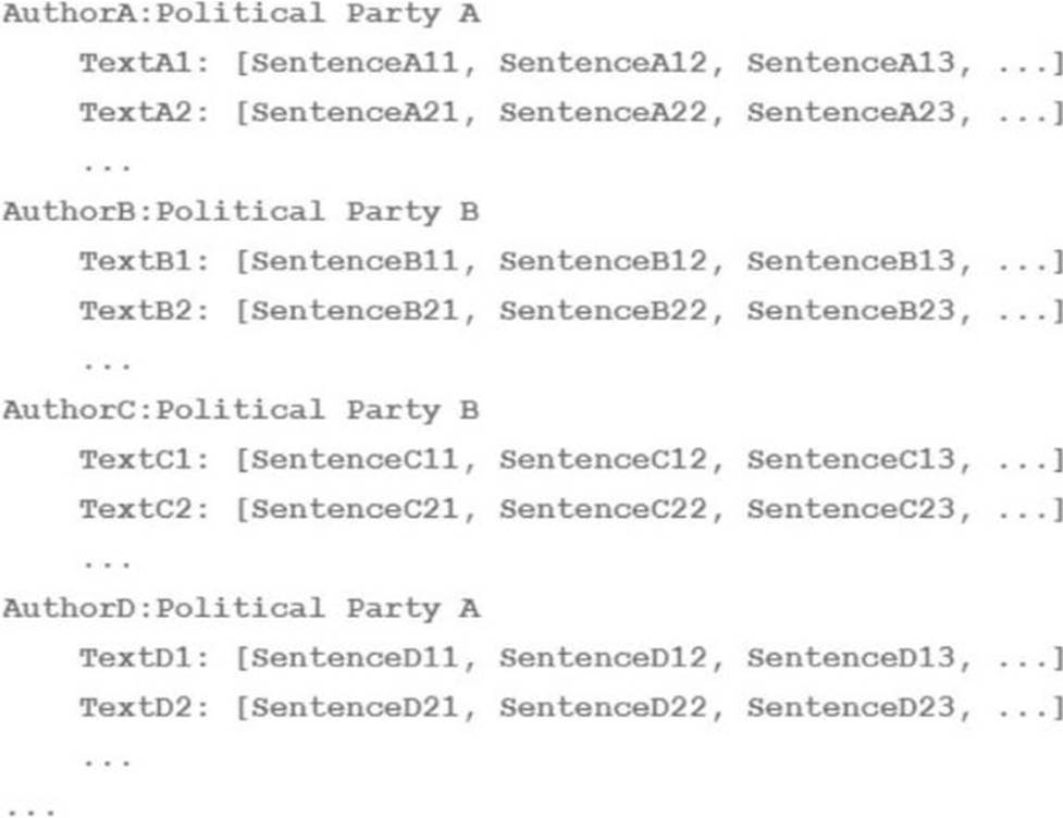
You followed the standard 80%-10%-10% data distribution across the training, testing, and evaluation subsets.
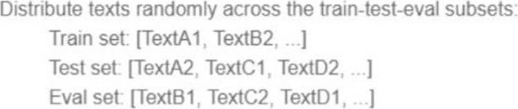
How should you distribute the training examples across the train-test-eval subsets while maintaining the 80-10-10 proportion?
A)
B)

C)

D)

- A . Option A
- B . Option B
- C . Option C
- D . Option D
C
Explanation:
The best way to distribute the training examples across the train-test-eval subsets while maintaining the 80-10-10 proportion is to use option C. This option ensures that each subset contains a balanced and representative sample of the different classes (Democrat and Republican) and the different authors. This way, the model can learn from a diverse and comprehensive set of articles and avoid overfitting or underfitting.
Option C also avoids the problem of data leakage, which occurs when the same author appears in more than one subset, potentially biasing the model and inflating its performance. Therefore, option C is the most suitable technique for this use case.