
Amazon MLS-C01 Practice Exams
Last updated on Oct 21,2026- Exam Code: MLS-C01
- Exam Name: AWS Certified Machine Learning - Specialty
- Certification Provider: Amazon
- Latest update: Oct 21,2026
A Machine Learning Specialist discover the following statistics while experimenting on a model.
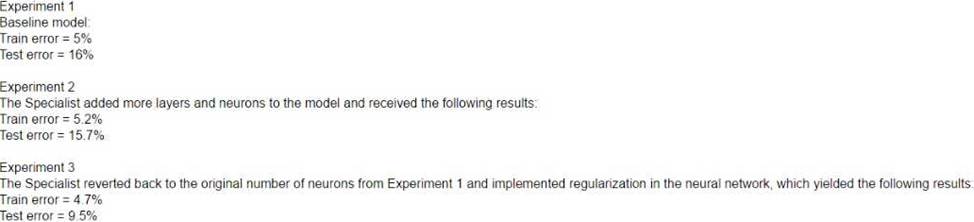
What can the Specialist from the experiments?
- A . The model In Experiment 1 had a high variance error that was reduced in Experiment 3 by regularization Experiment 2 shows that there is minimal bias error in Experiment 1
- B . The model in Experiment 1 had a high bias error that was reduced in Experiment 3 by regularization Experiment 2 shows that there is minimal variance error in Experiment 1
- C . The model in Experiment 1 had a high bias error and a high variance error that were reduced in Experiment 3 by regularization Experiment 2 shows that high bias cannot be reduced by increasing layers and neurons in the model
- D . The model in Experiment 1 had a high random noise error that was reduced in Experiment 3 by regularization Experiment 2 shows that random noise cannot be reduced by increasing layers and neurons in the model
A
Explanation:
The model in Experiment 1 had a high variance error because it performed well on the training data (train error = 5%) but poorly on the test data (test error = 8%). This indicates that the model was overfitting the training data and not generalizing well to new data. The model in Experiment 3 had a lower variance error because it performed similarly on the training data (train error = 5.1%) and the test data (test error = 5.4%). This indicates that the model was more robust and less sensitive to the fluctuations in the training data. The model in Experiment 3 achieved this improvement by implementing regularization, which is a technique that reduces the complexity of the model and prevents overfitting by adding a penalty term to the loss function. The model in Experiment 2 had a minimal bias error because it performed similarly on the training data (train error = 5.2%) and the test data (test error = 5.7%) as the model in Experiment 1. This indicates that the model was not underfitting the data and capturing the true relationship between the input and output variables. The model in Experiment 2 increased the number of layers and neurons in the model, which is a way to increase the complexity and flexibility of the model. However, this did not improve the performance of the model, as the variance error remained high. This shows that increasing the complexity of the model is not always the best way to reduce the bias error, and may even increase the variance error if the model becomes too complex for the data.
References:
Bias Variance Tradeoff – Clearly Explained – Machine Learning Plus. The Bias-Variance Trade-off in Machine Learning – Stack Abuse
A Machine Learning Specialist is building a logistic regression model that will predict whether or not a person will order a pizza. The Specialist is trying to build the optimal model with an ideal classification threshold.
What model evaluation technique should the Specialist use to understand how different classification
thresholds will impact the model’s performance?
- A . Receiver operating characteristic (ROC) curve
- B . Misclassification rate
- C . Root Mean Square Error (RM&)
- D . L1 norm
A
Explanation:
A receiver operating characteristic (ROC) curve is a model evaluation technique that can be used to understand how different classification thresholds will impact the model’s performance. A ROC curve plots the true positive rate (TPR) against the false positive rate (FPR) for various values of the classification threshold. The TPR, also known as sensitivity or recall, is the proportion of positive instances that are correctly classified as positive. The FPR, also known as the fall-out, is the proportion of negative instances that are incorrectly classified as positive. A ROC curve can show the trade-off between the TPR and the FPR for different thresholds, and help the Machine Learning Specialist to select the optimal threshold that maximizes the TPR and minimizes the FPR. A ROC curve can also be used to compare the performance of different models by calculating the area under the curve (AUC), which is a measure of how well the model can distinguish between the positive and negative classes. A higher AUC indicates a better model
A Machine Learning Specialist works for a credit card processing company and needs to predict which transactions may be fraudulent in near-real time. Specifically, the Specialist must train a model that returns the probability that a given transaction may be fraudulent.
How should the Specialist frame this business problem’?
- A . Streaming classification
- B . Binary classification
- C . Multi-category classification
- D . Regression classification
B
Explanation:
Binary classification is a type of supervised learning problem where the goal is to predict a categorical label that has only two possible values, such as Yes or No, True or False, Positive or Negative. In this case, the label is whether a transaction is fraudulent or not, which is a binary outcome. Binary classification can be used to estimate the probability of an observation belonging to a certain class, such as the probability of a transaction being fraudulent. This can help the business to make decisions based on the risk level of each transaction.
References:
Binary Classification – Amazon Machine Learning
AWS Certified Machine Learning – Specialty Sample Questions
A company wants to segment a large group of customers into subgroups based on shared characteristics. The company’s data scientist is planning to use the Amazon SageMaker built-in k-means clustering algorithm for this task. The data scientist needs to determine the optimal number of subgroups (k) to use.
Which data visualization approach will MOST accurately determine the optimal value of k?
- A . Calculate the principal component analysis (PCA) components. Run the k-means clustering algorithm for a range of k by using only the first two PCA components. For each value of k, create a scatter plot with a different color for each cluster. The optimal value of k is the value where the clusters start to look reasonably separated.
- B . Calculate the principal component analysis (PCA) components. Create a line plot of the number of components against the explained variance. The optimal value of k is the number of PCA components after which the curve starts decreasing in a linear fashion.
- C . Create a t-distributed stochastic neighbor embedding (t-SNE) plot for a range of perplexity values. The optimal value of k is the value of perplexity, where the clusters start to look reasonably separated.
- D . Run the k-means clustering algorithm for a range of k. For each value of k, calculate the sum of squared errors (SSE). Plot a line chart of the SSE for each value of k. The optimal value of k is the point after which the curve starts decreasing in a linear fashion.
D
Explanation:
The solution D is the best data visualization approach to determine the optimal value of k for the k-means clustering algorithm. The solution D involves the following steps:
Run the k-means clustering algorithm for a range of k. For each value of k, calculate the sum of squared errors (SSE). The SSE is a measure of how well the clusters fit the data. It is calculated by summing the squared distances of each data point to its closest cluster center. A lower SSE indicates a better fit, but it will always decrease as the number of clusters increases. Therefore, the goal is to find the smallest value of k that still has a low SSE1.
Plot a line chart of the SSE for each value of k. The line chart will show how the SSE changes as the value of k increases. Typically, the line chart will have a shape of an elbow, where the SSE drops rapidly at first and then levels off. The optimal value of k is the point after which the curve starts decreasing in a linear fashion. This point is also known as the elbow point, and it represents the balance between the number of clusters and the SSE1.
The other options are not suitable because:
Option A: Calculating the principal component analysis (PCA) components, running the k-means clustering algorithm for a range of k by using only the first two PCA components, and creating a scatter plot with a different color for each cluster will not accurately determine the optimal value of k. PCA is a technique that reduces the dimensionality of the data by transforming it into a new set of features that capture the most variance in the data. However, PCA may not preserve the original structure and distances of the data, and it may lose some information in the process. Therefore, running the k-means clustering algorithm on the PCA components may not reflect the true clusters in the data. Moreover, using only the first two PCA components may not capture enough variance to represent the data well. Furthermore, creating a scatter plot may not be reliable, as it depends on the subjective judgment of the data scientist to decide when the clusters look reasonably separated2.
Option B: Calculating the PCA components and creating a line plot of the number of components against the explained variance will not determine the optimal value of k. This approach is used to determine the optimal number of PCA components to use for dimensionality reduction, not for clustering. The explained variance is the ratio of the variance of each PCA component to the total variance of the data. The optimal number of PCA components is the point where adding more components does not significantly increase the explained variance. However, this number may not correspond to the optimal number of clusters, as PCA and k-means clustering have different objectives and assumptions2.
Option C: Creating a t-distributed stochastic neighbor embedding (t-SNE) plot for a range of perplexity values will not determine the optimal value of k. t-SNE is a technique that reduces the dimensionality of the data by embedding it into a lower-dimensional space, such as a two-dimensional plane. t-SNE preserves the local structure and distances of the data, and it can reveal clusters and patterns in the data. However, t-SNE does not assign labels or centroids to the clusters, and it does not provide a measure of how well the clusters fit the data. Therefore, t-SNE cannot determine the optimal number of clusters, as it only visualizes the data. Moreover, t-SNE depends on the perplexity parameter, which is a measure of how many neighbors each point considers. The perplexity parameter can affect the shape and size of the clusters, and there is no optimal value for it. Therefore, creating a t-SNE plot for a range of perplexity values may not be consistent or reliable3.
References:
1: How to Determine the Optimal K for K-Means?
2: Principal Component Analysis
3: t-Distributed Stochastic Neighbor Embedding
A machine learning specialist works for a fruit processing company and needs to build a system that categorizes apples into three types. The specialist has collected a dataset that contains 150 images for each type of apple and applied transfer learning on a neural network that was pretrained on ImageNet with this dataset.
The company requires at least 85% accuracy to make use of the model.
After an exhaustive grid search, the optimal hyperparameters produced the following:
68% accuracy on the training set
67% accuracy on the validation set
What can the machine learning specialist do to improve the system’s accuracy?
- A . Upload the model to an Amazon SageMaker notebook instance and use the Amazon SageMaker HPO feature to optimize the model’s hyperparameters.
- B . Add more data to the training set and retrain the model using transfer learning to reduce the bias.
- C . Use a neural network model with more layers that are pretrained on ImageNet and apply transfer learning to increase the variance.
- D . Train a new model using the current neural network architecture.
B
Explanation:
The problem described in the question is a case of underfitting, where the neural network model performs poorly on both the training and validation sets. This means that the model has not learned the features of the data well enough and has high bias.
To solve this issue, the machine learning specialist should consider the following change:
Add more data to the training set and retrain the model using transfer learning to reduce the bias:
Adding more data to the training set can help the model learn more patterns and variations in the data and improve its performance. Transfer learning can also help the model leverage the knowledge from the pre-trained network and adapt it to the new data. This can reduce the bias and increase the accuracy of the model.
References:
Transfer learning for TensorFlow image classification models in Amazon SageMaker
Transfer learning for custom labels using a TensorFlow container and “bring your own algorithm” in Amazon SageMaker
Machine Learning Concepts – AWS Training and Certification
A Data Scientist is developing a machine learning model to predict future patient outcomes based on information collected about each patient and their treatment plans. The model should output a continuous value as its prediction. The data available includes labeled outcomes for a set of 4,000 patients. The study was conducted on a group of individuals over the age of 65 who have a particular disease that is known to worsen with age.
Initial models have performed poorly. While reviewing the underlying data, the Data Scientist notices that, out of 4,000 patient observations, there are 450 where the patient age has been input as 0. The other features for these observations appear normal compared to the rest of the sample population.
How should the Data Scientist correct this issue?
- A . Drop all records from the dataset where age has been set to 0.
- B . Replace the age field value for records with a value of 0 with the mean or median value from the dataset.
- C . Drop the age feature from the dataset and train the model using the rest of the features.
- D . Use k-means clustering to handle missing features.
B
Explanation:
The best way to handle the missing values in the patient age feature is to replace them with the
mean or median value from the dataset. This is a common technique for imputing missing values
that preserves the overall distribution of the data and avoids introducing bias or reducing the sample
size. Dropping the records or the feature would result in losing valuable information and reducing the accuracy of the model. Using k-means clustering would not be appropriate for handling missing values in a single feature, as it is a method for grouping similar data points based on multiple features.
References:
Effective Strategies to Handle Missing Values in Data Analysis
How To Handle Missing Values In Machine Learning Data With Weka.
How to handle missing values in Python – Machine Learning Plus
A data scientist wants to use Amazon Forecast to build a forecasting model for inventory demand for a retail company. The company has provided a dataset of historic inventory demand for its products as a .csv file stored in an Amazon S3 bucket.
The table below shows a sample of the dataset.

How should the data scientist transform the data?
- A . Use ETL jobs in AWS Glue to separate the dataset into a target time series dataset and an item metadata dataset. Upload both datasets as .csv files to Amazon S3.
- B . Use a Jupyter notebook in Amazon SageMaker to separate the dataset into a related time series dataset and an item metadata dataset. Upload both datasets as tables in Amazon Aurora.
- C . Use AWS Batch jobs to separate the dataset into a target time series dataset, a related time series dataset, and an item metadata dataset. Upload them directly to Forecast from a local machine.
- D . Use a Jupyter notebook in Amazon SageMaker to transform the data into the optimized protobuf recordIO format. Upload the dataset in this format to Amazon S3.
A
Explanation:
Amazon Forecast requires the input data to be in a specific format. The data scientist should use ETL jobs in AWS Glue to separate the dataset into a target time series dataset and an item metadata dataset. The target time series dataset should contain the timestamp, item_id, and demand columns, while the item metadata dataset should contain the item_id, category, and lead_time columns. Both datasets should be uploaded as .csv files to Amazon S3.
References:
How Amazon Forecast Works – Amazon Forecast
Choosing Datasets – Amazon Forecast
A Machine Learning Specialist needs to create a data repository to hold a large amount of time-based training data for a new model. In the source system, new files are added every hour Throughout a single 24-hour period, the volume of hourly updates will change significantly. The Specialist always wants to train on the last 24 hours of the data
Which type of data repository is the MOST cost-effective solution?
- A . An Amazon EBS-backed Amazon EC2 instance with hourly directories
- B . An Amazon RDS database with hourly table partitions
- C . An Amazon S3 data lake with hourly object prefixes
- D . An Amazon EMR cluster with hourly hive partitions on Amazon EBS volumes
C
Explanation:
An Amazon S3 data lake is a cost-effective solution for storing and analyzing large amounts of time-based training data for a new model. Amazon S3 is a highly scalable, durable, and secure object storage service that can store any amount of data in any format. Amazon S3 also offers low-cost storage classes, such as S3 Standard-IA and S3 One Zone-IA, that can reduce the storage costs for infrequently accessed data. By using hourly object prefixes, the Machine Learning Specialist can organize the data into logical partitions based on the time of ingestion. This can enable efficient data access and management, as well as support incremental updates and deletes. The Specialist can also use Amazon S3 lifecycle policies to automatically transition the data to lower-cost storage classes or delete the data after a certain period of time. This way, the Specialist can always train on the last 24 hours of the data and optimize the storage costs.
Reference: What is a data lake? – Amazon Web Services
Amazon S3 Storage Classes – Amazon Simple Storage Service Managing your storage lifecycle – Amazon Simple Storage Service Best Practices Design Patterns: Optimizing Amazon S3 Performance
A Machine Learning team uses Amazon SageMaker to train an Apache MXNet handwritten digit classifier model using a research dataset. The team wants to receive a notification when the model is overfitting. Auditors want to view the Amazon SageMaker log activity report to ensure there are no unauthorized API calls.
What should the Machine Learning team do to address the requirements with the least amount of code and fewest steps?
- A . Implement an AWS Lambda function to long Amazon SageMaker API calls to Amazon S3. Add code to push a custom metric to Amazon CloudWatch. Create an alarm in CloudWatch with Amazon SNS to receive a notification when the model is overfitting.
- B . Use AWS CloudTrail to log Amazon SageMaker API calls to Amazon S3. Add code to push a custom metric to Amazon CloudWatch. Create an alarm in CloudWatch with Amazon SNS to receive a notification when the model is overfitting.
- C . Implement an AWS Lambda function to log Amazon SageMaker API calls to AWS CloudTrail. Add code to push a custom metric to Amazon CloudWatch. Create an alarm in CloudWatch with Amazon SNS to receive a notification when the model is overfitting.
- D . Use AWS CloudTrail to log Amazon SageMaker API calls to Amazon S3. Set up Amazon SNS to receive a notification when the model is overfitting.
B
Explanation:
To log Amazon SageMaker API calls, the team can use AWS CloudTrail, which is a service that provides a record of actions taken by a user, role, or an AWS service in SageMaker1. CloudTrail captures all API calls for SageMaker, with the exception of InvokeEndpoint and InvokeEndpointAsync, as events1. The calls captured include calls from the SageMaker console and code calls to the SageMaker API operations1. The team can create a trail to enable continuous delivery of CloudTrail events to an Amazon S3 bucket, and configure other AWS services to further analyze and act upon the event data collected in CloudTrail logs1. The auditors can view the CloudTrail log activity report in the CloudTrail console or download the log files from the S3 bucket1.
To receive a notification when the model is overfitting, the team can add code to push a custom metric to Amazon CloudWatch, which is a service that provides monitoring and observability for AWS resources and applications2. The team can use the MXNet metric API to define and compute the custom metric, such as the validation accuracy or the validation loss, and use the boto3 CloudWatch client to put the metric data to CloudWatch3. The team can then create an alarm in CloudWatch with Amazon SNS to receive a notification when the custom metric crosses a threshold that indicates overfitting.
For example, the team can set the alarm to trigger when the validation loss increases for a certain number of consecutive periods, which means the model is learning the noise in the training data and not generalizing well to the validation data.
References:
1: Log Amazon SageMaker API Calls with AWS CloudTrail – Amazon SageMaker
2: What Is Amazon CloudWatch? – Amazon CloudWatch
3: Metric API ― Apache MXNet documentation
: CloudWatch ― Boto 3 Docs 1.20.21 documentation
: Creating Amazon CloudWatch Alarms – Amazon CloudWatch
: What is Amazon Simple Notification Service? – Amazon Simple Notification Service
: Overfitting and Underfitting – Machine Learning Crash Course
A Machine Learning Specialist previously trained a logistic regression model using scikit-learn on a local machine, and the Specialist now wants to deploy it to production for inference only.
What steps should be taken to ensure Amazon SageMaker can host a model that was trained locally?
- A . Build the Docker image with the inference code. Tag the Docker image with the registry hostname and upload it to Amazon ECR.
- B . Serialize the trained model so the format is compressed for deployment. Tag the Docker image with the registry hostname and upload it to Amazon S3.
- C . Serialize the trained model so the format is compressed for deployment. Build the image and upload it to Docker Hub.
- D . Build the Docker image with the inference code. Configure Docker Hub and upload the image to Amazon ECR.
A
Explanation:
To deploy a model that was trained locally to Amazon SageMaker, the steps are:
Build the Docker image with the inference code. The inference code should include the model loading, data preprocessing, prediction, and postprocessing logic. The Docker image should also include the dependencies and libraries required by the inference code and the model.
Tag the Docker image with the registry hostname and upload it to Amazon ECR. Amazon ECR is a fully managed container registry that makes it easy to store, manage, and deploy container images. The registry hostname is the Amazon ECR registry URI for your account and Region. You can use the AWS CLI or the Amazon ECR console to tag and push the Docker image to Amazon ECR.
Create a SageMaker model entity that points to the Docker image in Amazon ECR and the model artifacts in Amazon S3. The model entity is a logical representation of the model that contains the information needed to deploy the model for inference. The model artifacts are the files generated by the model training process, such as the model parameters and weights. You can use the AWS CLI, the SageMaker Python SDK, or the SageMaker console to create the model entity.
Create an endpoint configuration that specifies the instance type and number of instances to use for hosting the model. The endpoint configuration also defines the production variants, which are the different versions of the model that you want to deploy. You can use the AWS CLI, the SageMaker Python SDK, or the SageMaker console to create the endpoint configuration.
Create an endpoint that uses the endpoint configuration to deploy the model. The endpoint is a web
service that exposes an HTTP API for inference requests. You can use the AWS CLI, the SageMaker Python SDK, or the SageMaker console to create the endpoint.
References:
AWS Machine Learning Specialty Exam Guide
AWS Machine Learning Training – Deploy a Model on Amazon SageMaker
AWS Machine Learning Training – Use Your Own Inference Code with Amazon SageMaker Hosting Services